Dirac Delta Function — Question 1

PDF ↗

Question 1

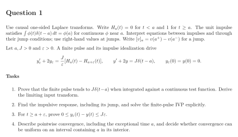
Use causal one-sided Laplace transforms. Write Ha(t)=0H_a(t)=0 for t<at<a and 11 for t≥at\ge a. The unit impulse satisfies ∫ϕ(t)δ(t−a)dt=ϕ(a)\int\phi(t)\delta(t-a)\,dt=\phi(a) for continuous ϕ\phi near aa. Interpret equations between impulses and through their jump conditions; use right-hand values at jumps. Write [v]a=v(a+)−v(a−)[v]_a=v(a^+)-v(a^-) for a jump.

Let a,J>0a,J>0 and ε>0\varepsilon>0. A finite pulse and its impulse idealization drive yε′+2yε=Jε[Ha(t)−Ha+ε(t)],y′+2y=Jδ(t−a),yε(0)=y(0)=0.y_\varepsilon'+2y_\varepsilon =\frac J\varepsilon[H_a(t)-H_{a+\varepsilon}(t)], \qquad y'+2y=J\delta(t-a),\qquad y_\varepsilon(0)=y(0)=0.

Tasks

  1. Prove that the finite pulse tends to Jδ(t−a)J\delta(t-a) when integrated against a continuous test function. Derive the limiting input transform.

  2. Find the impulsive response, including its jump, and solve the finite-pulse IVP explicitly.

  3. For t≥a+εt\ge a+\varepsilon, prove 0≤yε(t)−y(t)≤Jε0\le y_\varepsilon(t)-y(t)\le J\varepsilon.

  4. Describe pointwise convergence, including the exceptional time aa, and decide whether convergence can be uniform on an interval containing aa in its interior.

Original worksheet page 1: question and worked solution for 4-8-001
Show solutionHide solution

Question 1 – Solution

Strategy. Preserve pulse area rather than height. Compare the two exact responses before making any claim about convergence.

Step 1: Test the pulse and transform. Its action on a continuous ϕ\phi is Jε∫aa+εϕ(t)dt→Jϕ(a).\frac J\varepsilon\int_a^{a+\varepsilon}\phi(t)\,dt \longrightarrow J\phi(a). The error is at most Jsup⁡[a,a+ε]|ϕ(t)−ϕ(a)|J\sup_{[a,a+\varepsilon]}|\phi(t)-\phi(a)|, which tends to zero. Taking ϕ=e−st\phi=e^{-st} gives Fε=Je−as(1−e−εs)/(εs)→Je−asF_\varepsilon=Je^{-as}(1-e^{-\varepsilon s})/(\varepsilon s)\to Je^{-as}, with the removable value Fε(0)=JF_\varepsilon(0)=J.

Step 2: Solve both equations. The impulse gives Y=Je−as/(s+2)Y=Je^{-as}/(s+2), so y=JHa(t)e−2(t−a)\boxed{y=JH_a(t)e^{-2(t-a)}} and [y]a=J[y]_a=J. The finite-pulse solution is continuous and equals yε(t)={0,t<a,J2ε(1−e−2(t−a)),a≤t<a+ε,J2ε(1−e−2ε)e−2(t−a−ε),t≥a+ε.y_\varepsilon(t)=\begin{cases} 0,&t<a,\\ \dfrac{J}{2\varepsilon}(1-e^{-2(t-a)}),&a\le t<a+\varepsilon,\\ \dfrac{J}{2\varepsilon}(1-e^{-2\varepsilon}) e^{-2(t-a-\varepsilon)},&t\ge a+\varepsilon. \end{cases} Each piece satisfies its ordinary equation, and the endpoints match.

Step 3: Bound the tail error. Put τ=t−a≥ε\tau=t-a\ge\varepsilon. The explicit tail can be rewritten as yε=(J/ε)∫0εe−2(τ−u)duy_\varepsilon=(J/\varepsilon)\int_0^\varepsilon e^{-2(\tau-u)}\,du. Since x↦e−2xx\mapsto e^{-2x} is decreasing and has derivative magnitude at most 22 for x≥0x\ge 0, 0≤yε−y=Jε∫0ε[e−2(τ−u)−e−2τ]du≤Jε∫0ε2udu=Jε.0\le y_\varepsilon-y =\frac J\varepsilon\int_0^\varepsilon [e^{-2(\tau-u)}-e^{-2\tau}]\,du \le\frac J\varepsilon\int_0^\varepsilon 2u\,du =\boxed{J\varepsilon}. This representation follows directly from the finite-pulse formula.

Step 4: Distinguish the kinds of convergence. For each fixed t≠at\ne a, yε(t)→y(t)y_\varepsilon(t)\to y(t). At aa, yε(a)=0y_\varepsilon(a)=0 but the right-hand representative has y(a)=Jy(a)=J. Uniform convergence on an interval containing aa is impossible: the approximants are continuous and the limit has a jump. Changing only y(a)y(a) does not remove that jump or change its transform. The graph uses a=J=1a=J=1; open and filled dots mark the impulsive response.

See the diagram in the original worksheet below.

Original worksheet page 2: question and worked solution for 4-8-001

Original worksheet layout. Use Enlarge or open the PDF for a closer view.