Question 10
Use causal one-sided Laplace transforms. Write for and for . The unit impulse satisfies for continuous near . Interpret equations between impulses and through their jump conditions; use right-hand values at jumps. Write for a jump.
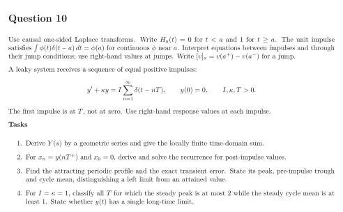
A leaky system receives a sequence of equal positive impulses: The first impulse is at , not at zero. Use right-hand response values at each impulse.
Tasks
Derive by a geometric series and give the locally finite time-domain sum.
For and , derive and solve the recurrence for post-impulse values.
Find the attracting periodic profile and the exact transient error. State its peak, pre-impulse trough and cycle mean, distinguishing a left limit from an attained value.
For , classify all for which the steady peak is at most while the steady cycle mean is at least . State whether has a single long-time limit.
Show solutionHide solution
Question 10 – Solution
Strategy. Each impulse adds to the state, while the gap between impulses multiplies it by an exponential. The cycle map determines the limiting profile.
Step 1: Sum the transforms and invert. For , the impulse series converges geometrically: Thus Only finitely many terms are active at each time. The formula gives zero before , jumps of , and between impulses.
Step 2: Solve the post-impulse recurrence. Put . Decay followed by a jump gives The steady post-impulse level is .
Step 3: Construct the profile and compare. For , , define . Then , including , and The profile’s peak is attained just after each impulse. Its pre-impulse trough is the left limit ; under the right-hand convention this infimum is not attained within a cycle. Its mean is The jump is preserved in the limit, not smoothed away.
Step 4: Design a feasible spacing and interpret. With , the peak constraint gives , equivalent to . The mean constraint gives , equivalent to . Therefore There is no single long-time limit: samples at tend to , while samples at tend to the different value . Both responses have exact real transform domain because their persistent positive cycles prevent convergence at or below zero. The plot uses and marks the jump endpoints explicitly.
See the diagram in the original worksheet below.
