Question 10
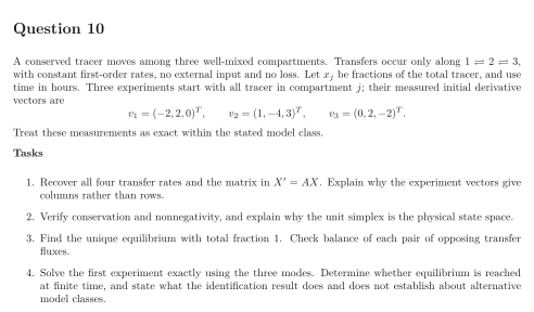
A conserved tracer moves among three well-mixed compartments. Transfers occur only along , with constant first-order rates, no external input and no loss. Let be fractions of the total tracer, and use time in hours. Three experiments start with all tracer in compartment ; their measured initial derivative vectors are Treat these measurements as exact within the stated model class.
Tasks
Recover all four transfer rates and the matrix in . Explain why the experiment vectors give columns rather than rows.
Verify conservation and nonnegativity, and explain why the unit simplex is the physical state space.
Find the unique equilibrium with total fraction . Check balance of each pair of opposing transfer fluxes.
Solve the first experiment exactly using the three modes. Determine whether equilibrium is reached at finite time, and state what the identification result does and does not establish about alternative model classes.
Show solutionHide solution
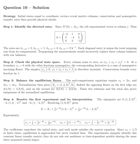
Question 10 – Solution
Strategy. Initial states equal to coordinate vectors reveal matrix columns; conservation and nonnegative transfer rates then provide physical checks.
Step 1: Identify the directed rates. Since , the th experimental vector is column . Thus The rates are , , , h. Each diagonal entry is minus the total outgoing rate from its compartment. Transposing the measurements would incorrectly replace these column balances with row balances.
Step 2: Check the physical state space. Every column sums to zero, so . At a boundary with the other fractions nonnegative, the corresponding derivative is a sum of nonnegative incoming fluxes. The simplex is therefore invariant. Conservation bounds every fraction by .
Step 3: Balance the equilibrium fluxes. The end-compartment equations require and . Normalization then gives . Indeed the opposing fluxes on the first edge are , and on the second are . These two relations and the total also prove uniqueness of the normalized equilibrium.
Step 4: Resolve the first experiment and its interpretation. The eigenpairs are , and . Resolving gives Equivalently, The coefficients reproduce the initial state, and each mode satisfies the matrix equation. Since at finite times, equilibrium is approached but never reached then. The experiments uniquely identify this constant linear transfer matrix; they do not rule out nonlinear or time-dependent models sharing the same three measured initial slopes.