Terminology — Question 3

Question 3 – Solution

Strategy. Identify both the operator being prescribed and the geometric location of the data.

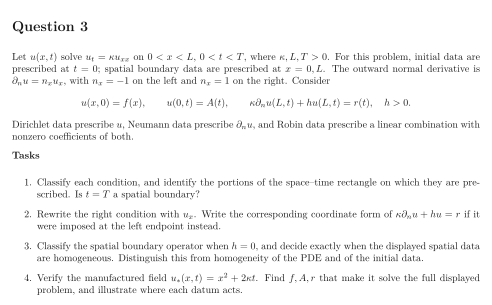
Step 1: Locate and name the data. The bottom edge $t=0$ carries initial displacement/temperature data $f(x)$. The left edge carries Dirichlet data $A(t)$; the right carries Robin data $r(t)$. The top $t=T$ is a final-time slice, not a spatial boundary. No data are prescribed there in this initial-boundary-value problem.

Step 2: Keep the outward signs. At the right, the condition is $\kappa u_x(L,t)+h u(L,t)=r(t)$. At the left, the analogous outward-normal condition would be $-\kappa u_x(0,t)+h u(0,t)=r(t)$. Changing the endpoint changes the sign of the normal derivative, not the sign of the prescribed value by convention.

Step 3: Classify homogeneity at each level. When $h=0$, the right condition is Neumann, since $\kappa>0$. The spatial data are homogeneous exactly when $A\equiv 0$ and $r\equiv 0$. The PDE is already linear homogeneous; initial data are homogeneous exactly when $f\equiv 0$. These are three separate assertions. A nonzero Robin coefficient $h$ does not itself make the condition nonhomogeneous.

Step 4: Verify all parts of a full problem. Here $u_{*,t}=2\kappa$ and $u_{*,xx}=2$, so the PDE holds. Evaluation gives $$\boxed{f(x)=x^2,\quad A(t)=2\kappa t,\quad r(t)=2\kappa L+h(L^2+2\kappa t).}$$ These data also agree at their shared corners. The diagram locates the data; it is a space–time domain, not a graph of the solution value.