Solving the Heat Equation — Question 5

Question 5 – Solution

Strategy. Insulation preserves the constant component while all nonconstant cosine modes decay.

Step 1: Compute and evolve the cosine coefficients. Integration gives $a_0=L/2$ and $a_n=2L(({-1})^n-1)/(\pi^2n^2)$. Therefore $$\boxed{u(x,t)=\frac L2-\frac{4L}{\pi^2}\sum_{n\text{ odd}} \frac{e^{-\kappa(n\pi/L)^2t}\cos(n\pi x/L)}{n^2}.}$$ Gaussian decay justifies the PDE and derivative boundary conditions termwise for $t>0$. The constant mode remains stationary.

Step 2: Identify the conserved and symmetric parts. Integrating the PDE yields $(\int u)'=\kappa[u_x]_0^L=0$, so the mean is $L/2$. For odd $n$, $\cos(n\pi(L-x)/L)=-\cos(n\pi x/L)$. The series therefore gives $u(L-x,t)=L-u(x,t)$, in particular $u(L/2,t)=L/2$ at all times. The absolutely summable coefficients and positive modal decay imply uniform convergence to the equilibrium $L/2$ as $t\to\infty$.

Step 3: Check values and derivatives separately. The $n^{-2}$ coefficients give absolute uniform convergence at $t=0$; the cosine convergence theorem identifies the sum as $x$, including both endpoints. Summable domination proves uniform recovery of those values as $t\downarrow 0$. But the initial trace has derivative one, whereas $u_x=0$ at the endpoints for every positive time. A continuously extending spatial derivative would have to take both values at each initial corner, which is impossible. Uniform convergence of temperatures does not imply convergence of derivatives.

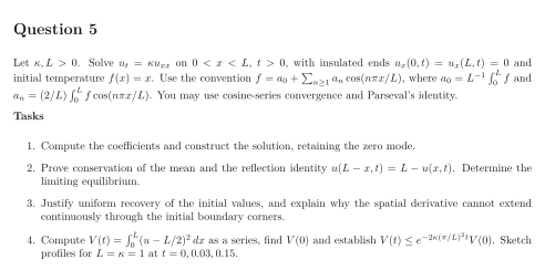
Step 4: Quantify equilibration. Orthogonality gives $$V(t)=\frac{8L^3}{\pi^4}\sum_{n\text{ odd}}\frac{e^{-2\kappa(n\pi/L)^2t}}{n^4}, \qquad V(0)=\int_0^L(x-L/2)^2\,dx=\frac{L^3}{12}.$$ Each exponential is at most $e^{-2\kappa(\pi/L)^2t}$, proving the required bound. The profiles flatten toward their conserved mean, rather than toward zero. Only the initial profile has the incompatible endpoint slopes.