Heat Equation with Non-Zero Temperature Boundaries — Question 6

Question 6 – Solution

Strategy. A periodic boundary signal diffuses inward with both amplitude attenuation and a spatial phase shift.

Step 1: Match the PDE and the initial trace. Put $\theta=\omega t-\alpha x$. Then $u_t=-\omega B e^{-\alpha x}\sin\theta$ and $u_{xx}=-2\alpha^2B e^{-\alpha x}\sin\theta$. Thus $\boxed{\alpha=\sqrt{\omega/(2\kappa)}}$. The boundary trace is the imposed cosine, and the compatible initial field is $f(x)=A+B e^{-\alpha x}\cos(\alpha x)$. It is generally not the constant $A$; a constant initial field would require an additional transient.

Step 2: Quantify attenuation and delay. The local oscillation amplitude is $|B|e^{-\alpha x}$ and its phase lag is $\alpha x$. Relative to the boundary waveform, the time delay is $\alpha x/\omega$, understood modulo the period. The penetration depth is $$\boxed{d=1/\alpha=\sqrt{2\kappa/\omega}=\sqrt{\kappa P/\pi}.}$$ Longer periods penetrate farther, with depth proportional to the square root of the period rather than the period itself.

Step 3: Determine the phase of the boundary flux. Differentiation gives $u_x=\alpha B e^{-\alpha x}(-\cos\theta+\sin\theta)$. Hence $$\boxed{j(0,t)=B\sqrt{\kappa\omega}\cos(\omega t+\pi/4).}$$ The flux leads the boundary temperature oscillation by $\pi/4$ in phase and has zero average over a full period. Instantaneous storage and release near the driven boundary are compatible with a constant far-field limit.

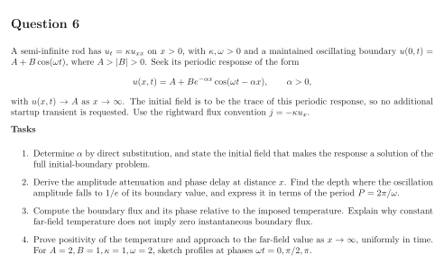
Step 4: Verify bounds and interpret the profiles. For all $x\ge 0,t$, $|u-A|\le|B|e^{-\alpha x}\le|B|$, so $u\ge A-|B|>0$. Also $\sup_t|u(x,t)-A|\le|B|e^{-\alpha x}\to 0$ as $x\to\infty$. This is a spatial far-field limit uniform in time, not decay of the maintained oscillation at a fixed point as time increases. For the plotted parameters, $\alpha=1$ and the penetration depth is one.