Question 10
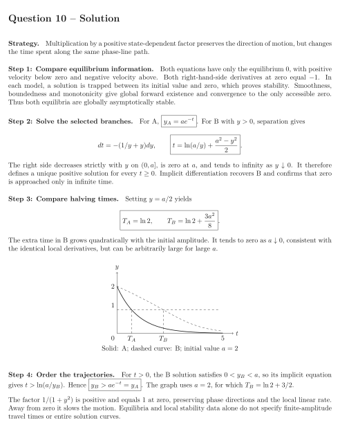
Compare two autonomous equations on the real line: For the quantitative comparison, use the same initial value .
Tasks
Compare the equilibrium sets, phase-line arrows and derivatives of the right-hand sides at the equilibria. Prove the stability classification for both equations.
Find the solution of A and an implicit relation for B. Justify global forward existence and convergence for B.
Derive the time required to decrease from to for each equation. Explain how the difference depends on .
For , sketch both trajectories and determine which is larger for every . Explain what identical equilibrium and local derivative data fail to specify.
Show solutionHide solution
Question 10 – Solution
Strategy. Multiplication by a positive state-dependent factor preserves the direction of motion, but changes the time spent along the same phase-line path.
Step 1: Compare equilibrium information. Both equations have only the equilibrium , with positive velocity below zero and negative velocity above. Both right-hand-side derivatives at zero equal . In each model, a solution is trapped between its initial value and zero, which proves stability. Smoothness, boundedness and monotonicity give global forward existence and convergence to the only accessible zero. Thus both equilibria are globally asymptotically stable.
Step 2: Solve the selected branches. For A, . For B with , separation gives The right side decreases strictly with on , is zero at , and tends to infinity as . It therefore defines a unique positive solution for every . Implicit differentiation recovers B and confirms that zero is approached only in infinite time.
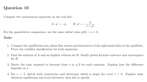
Step 3: Compare halving times. Setting yields The extra time in B grows quadratically with the initial amplitude. It tends to zero as , consistent with the identical local derivatives, but can be arbitrarily large for large .
See the diagram in the original worksheet below.
Step 4: Order the trajectories. For , the B solution satisfies , so its implicit equation gives . Hence . The graph uses , for which .
The factor is positive and equals at zero, preserving phase directions and the local linear rate. Away from zero it slows the motion. Equilibria and local stability data alone do not specify finite-amplitude travel times or entire solution curves.