Table Of Laplace Transforms — Question 6

Question 6 – Solution

Strategy. A one-cycle transform and a geometric series supply the periodic row; delayed ramps independently encode its slope changes.

Step 1: Sum the cycles. For $s>0$, boundedness gives absolute convergence. Splitting into intervals $[2n,2n+2]$ and translating yields $$P(s)=\frac{\int_0^2e^{-st}p(t)\,dt}{1-e^{-2s}} =\boxed{\frac{(1-e^{-s})^2}{s^2(1-e^{-2s})} =\frac{1-e^{-s}}{s^2(1+e^{-s})}.}$$ The one-cycle integral is $(1-e^{-s})^2/s^2$, obtained by integration by parts on $[0,1]$ and $[1,2]$.

Step 2: Recover the slope changes. Write $R_a=(t-a)H_a(t)$. The series $$p(t)=\sum_{n=0}^\infty[R_{2n}-2R_{2n+1}+R_{2n+2}]$$ is locally finite; each bracket is a unit triangular pulse on $[2n,2n+2]$. Its transform is $e^{-2ns}(1-2e^{-s}+e^{-2s})/s^2$. Summing for $s>0$ gives the same $P$. These brackets, rather than the individual growing ramps across all cycles, also make absolute convergence clear.

Step 3: Check convergence and the mean. The signal is bounded, nonnegative and has area $1$ per period. Thus the exact real domain is $s>0$: at $s=0$ the areas sum to infinity, and for $s<0$ the weighted cycle contributions grow. Using $(1-e^{-s})/(1+e^{-s})=\tanh(s/2)$, $\lim_{s\to 0^+}sP(s)=\boxed{1/2}$, the cycle mean $1/2$.

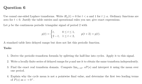
Step 4: Distinguish the limit notions. The samples $p(2n)=0$ and $p(2n+1)=1$ rule out a pointwise final value. Taylor expansion of the last quotient gives $$\boxed{P(s)=\frac 1{2s}-\frac{s}{24}+O(s^3).}$$ The leading pole records the mean, while the constant term vanishes. The figure displays continuous corners and equal successive cycles.