Question 6
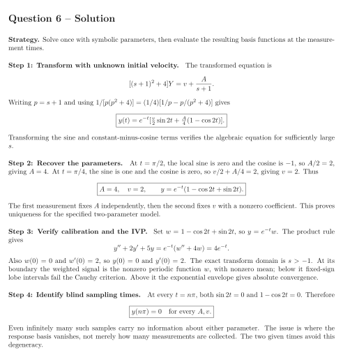
Use one-sided Laplace transforms and retain all initial-value terms. Write , with real sufficiently large during the transformation. Unless stated otherwise, solve on .
Two parameters are unknown in the IVP Exact measurements are and .
Tasks
Solve by Laplace transforms in terms of .
Use the two measurements to recover and prove uniqueness of this parameter recovery.
Verify the calibrated equation and both initial data. State the transform domain of the calibrated solution.
Would measurements taken only at , for positive integers , identify these parameters? Justify your answer from the exact response, not from a count of samples.
Show solutionHide solution
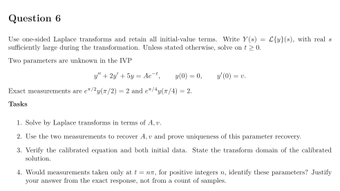
Question 6 – Solution
Strategy. Solve once with symbolic parameters, then evaluate the resulting basis functions at the measurement times.
Step 1: Transform with unknown initial velocity. The transformed equation is Writing and using gives Transforming the sine and constant-minus-cosine terms verifies the algebraic equation for sufficiently large .
Step 2: Recover the parameters. At , the local sine is zero and the cosine is , so , giving . At , the sine is one and the cosine is zero, so , giving . Thus The first measurement fixes independently, then the second fixes with a nonzero coefficient. This proves uniqueness for the specified two-parameter model.
Step 3: Verify calibration and the IVP. Set , so . The product rule gives Also and , so and . The exact transform domain is . At its boundary the weighted signal is the nonzero periodic function , with nonzero mean; below it fixed-sign lobe intervals fail the Cauchy criterion. Above it the exponential envelope gives absolute convergence.
Step 4: Identify blind sampling times. At every , both and . Therefore Even infinitely many such samples carry no information about either parameter. The issue is where the response basis vanishes, not merely how many measurements are collected. The two given times avoid this degeneracy.