Nonconstant Coefficient IVP’s — Question 10

Question 10 – Solution

Strategy. The data lost from the transform equation return as compatibility conditions on the forcing. Boundedness removes the singular time-domain homogeneous mode.

Step 1: Transform the time multipliers. The three left-hand terms transform to $-Y-sY'$, $-Y'$ and $2Y$. Thus $$\boxed{-(s+1)Y'+Y=\frac A{(s+1)^2}+\frac B{s+1}.}$$ The initial value in $sY-y(0)$ differentiates to zero in $\mathcal L\{ty'\}$. It must still be imposed on the inverse, not added back as a fictitious term.

Step 2: Solve and remove the inadmissible branch. Writing $p=s+1$, divide by $p^2$ to obtain $$(Y/p)'=-A/p^4-B/p^3.$$ Integration gives $$Y=\frac{A/3}{(s+1)^2}+\frac{B/2}{s+1}+C(s+1).$$ Decay requires $C=0$. The remaining terms invert to $\boxed{y=e^{-t}(At/3+B/2)}$, whose transform can now be verified directly.

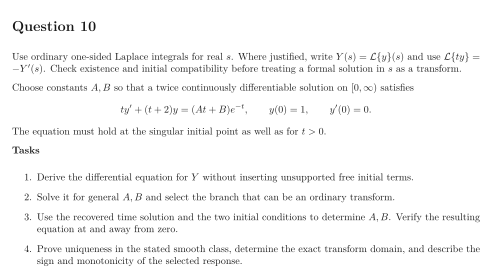
Step 3: Recover the forcing constants and verify. The initial value requires $B/2=1$, and the initial slope requires $A/3-B/2=0$. Hence $$\boxed{A=3,\quad B=2,\qquad y=(1+t)e^{-t}.}$$ Its derivative is $-te^{-t}$, so $$ty'+(t+2)y=e^{-t}[-t^2+(t+2)(1+t)]=(3t+2)e^{-t}.$$ At zero the equation gives $2y(0)=B$, and both specified data hold. The smooth extension also has $y''(0)=-1$.

Step 4: Prove uniqueness and check the response. For $t>0$, multiplying the original first-order equation by $te^t$ gives $(t^2e^t y)'=At^2+Bt$. Thus every local solution differs from the selected one by $K e^{-t}/t^2$. This mode is unbounded at zero unless $K=0$, proving uniqueness in the stated smooth class. The selected function is positive, with $y'<0$ for $t>0$, and decreases from one to zero after an initially horizontal tangent. Its positive polynomial-exponential tail gives exact transform domain $\boxed{s>-1}$. The parameter restrictions arise from compatibility, not from a regular existence theorem where the leading coefficient vanishes.