Question 1
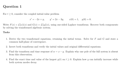
For , consider the coupled initial-value problem Write and , using one-sided Laplace transforms. Recover both components by solving the transformed algebraic system.
Tasks
Derive the two transformed equations, retaining the initial terms. Solve for and and state a common half-plane of convergence.
Invert both transforms and verify the initial values and original differential equations.
Find the transform and time response of . Explain why one pole of the full system is absent from this observation.
Find the exact time and value of the largest on . Explain how can initially increase while both system modes decay.
Show solutionHide solution
Question 1 – Solution
Strategy. Keep the initial data on the right side of the transformed system, then distinguish component responses from observed combinations.
Step 1: Solve the algebraic system. The derivative rule gives and . Their determinant is , so Both transforms converge for . Dropping the initial term would incorrectly give the zero solution.
Step 2: Invert and check. Partial fractions give At zero these are . Differentiation gives and , which equal and .
Step 3: Explain the cancelled pole. Subtracting the transforms gives , hence . The slow mode is a multiple of ; subtracting its components annihilates it. The state still contains this mode. Cancellation in an observation does not remove a mode from the system.
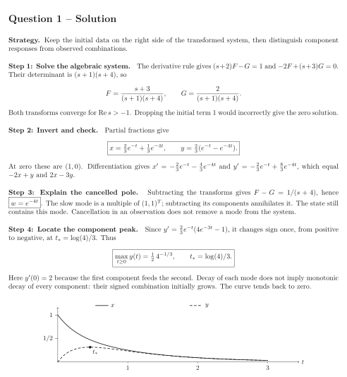
Step 4: Locate the component peak. Since , it changes sign once, from positive to negative, at . Thus Here because the first component feeds the second. Decay of each mode does not imply monotonic decay of every component: their signed combination initially grows. The curve tends back to zero.
See the diagram in the original worksheet below.