Question 5
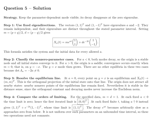
For a real parameter , consider Treat the zero-eigenvalue case explicitly; do not assume that every equilibrium is isolated.
Tasks
Find the eigenvalues, an eigenbasis independent of , and the solution with arbitrary initial state .
Classify the origin for and , and identify the initial states that converge to it in each case.
At , find every equilibrium and the limiting state of every solution. Is the origin attracting all nearby states?
For initial state , compare with . Explain the difference.
Show solutionHide solution
Question 5 – Solution
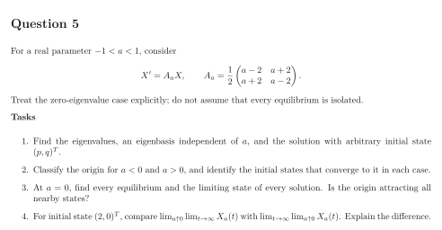
Strategy. Keep the parameter-dependent mode visible; its decay disappears at the zero eigenvalue.
Step 1: Use fixed eigendirections. The vectors and have eigenvalues and . They remain independent, and their eigenvalues are distinct throughout the stated parameter interval. Setting , gives This formula satisfies the system and the initial data for every allowed .
Step 2: Classify the nonzero-parameter cases. For , both modes decay, so the origin is a stable node and all initial states converge to it. For , the origin is a saddle; convergence occurs exactly when , that is, on . The mode then grows. There are no other equilibria in these two cases because .
Step 3: Resolve the equilibrium line. At , every point on is an equilibrium and . This is the orthogonal projection of the initial state onto that line. The origin does not attract all nearby states: nearby nonzero points of the equilibrium line remain fixed. Nevertheless it is stable in the distance sense, since the orthogonal constant and decaying modes never increase the Euclidean norm.
Step 4: Compare the orders of limiting. For the specified data, . At each fixed the time limit is zero; hence the first iterated limit is . At each fixed finite , taking instead gives , whose time limit is . The decay becomes arbitrarily slow as approaches zero from below. It is not uniform over such parameters on an unbounded time interval, so these two operations need not commute.