Heat Equation with Non-Zero Temperature Boundaries — Question 1

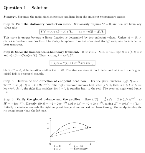
Question 1 – Solution

Strategy. Separate the maintained stationary gradient from the transient temperature excess.

Step 1: Find the stationary conduction state. Stationarity requires $S''=0$, and the two boundary values give $$\boxed{S(x)=A+(B-A)x/L,\qquad j_S=-\kappa(B-A)/L.}$$ This state is unique because a linear function is determined by two endpoint values. Unless $A=B$, it carries a constant nonzero flux. Stationary temperature means zero local storage rate, not an absence of heat transport.

Step 2: Solve the homogeneous-boundary transient. With $v=u-S$, $v_t=\kappa v_{xx}$, $v(0,t)=v(L,t)=0$ and $v(x,0)=C\sin(\pi x/L)$. Thus, writing $\lambda=\kappa\pi^2/L^2$, $$\boxed{u(x,t)=S(x)+Ce^{-\lambda t}\sin(\pi x/L).}$$ Since $S''=0$, differentiation verifies the PDE. The sine vanishes at both ends, and at $t=0$ the original initial field is recovered exactly.

Step 3: Determine the direction of endpoint heat flow. For the given numbers, $u_x(1,t)=2-2\pi e^{-\pi^2t}$, so $j(1,t)=-2+2\pi e^{-\pi^2t}$. The right reservoir receives heat when $j>0$, that is $0\le t<t_*:=\log\pi/\pi^2$. At $t_*$ the right flux vanishes; for $t>t_*$ it supplies heat to the rod. The eventual rightward flux is $-2$.

Step 4: Verify the global balance and the profiles. Here $H(t)=\int_0^1u\,dx=2+(4/\pi)e^{-\pi^2t}$, so $H'=-4\pi e^{-\pi^2t}$. Directly $j(0,t)=-2-2\pi e^{-\pi^2t}$ and $j(1,t)=-2+2\pi e^{-\pi^2t}$, giving $H'=j(0,t)-j(1,t)$. Initially the interior exceeds the right endpoint temperature, so heat can leave through that endpoint despite its being hotter than the left one.