Question 4
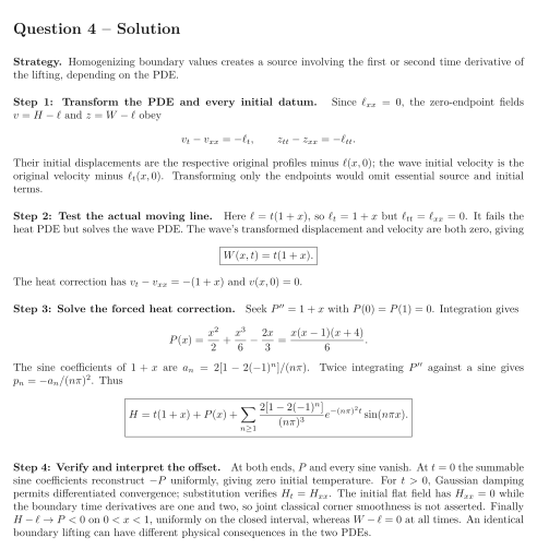
On , compare and with the moving boundary values Take and .
Tasks
For general boundary values , derive the transformed PDE and initial data after subtracting in each problem.
For the specified data, decide whether the affine lifting itself solves each original PDE.
Construct the complete heat solution using a stationary correction to its transformed forcing and a sine expansion. Derive the required coefficients.
Verify the reconstructed original data and find the long-time heat offset relative to the moving line. Contrast it with the wave field and state the heat release-corner regularity caveat.
Show solutionHide solution
Question 4 – Solution
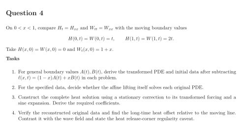
Strategy. Homogenizing boundary values creates a source involving the first or second time derivative of the lifting, depending on the PDE.
Step 1: Transform the PDE and every initial datum. Since , the zero-endpoint fields and obey Their initial displacements are the respective original profiles minus ; the wave initial velocity is the original velocity minus . Transforming only the endpoints would omit essential source and initial terms.
Step 2: Test the actual moving line. Here , so but . It fails the heat PDE but solves the wave PDE. The wave’s transformed displacement and velocity are both zero, giving The heat correction has and .
Step 3: Solve the forced heat correction. Seek with . Integration gives The sine coefficients of are . Twice integrating against a sine gives . Thus
Step 4: Verify and interpret the offset. At both ends, and every sine vanish. At the summable sine coefficients reconstruct uniformly, giving zero initial temperature. For , Gaussian damping permits differentiated convergence; substitution verifies . The initial flat field has while the boundary time derivatives are one and two, so joint classical corner smoothness is not asserted. Finally on , uniformly on the closed interval, whereas at all times. An identical boundary lifting can have different physical consequences in the two PDEs.