Question 3
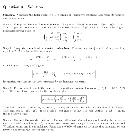
On , consider the Euler-type equation Use the proposed homogeneous basis and variation of parameters, rather than a guessed logarithmic trial.
Tasks
Verify the three homogeneous solutions and their Wronskian. Normalize the equation and write the parameter system with the correct right-hand side.
Solve for the parameter derivatives and integrate to obtain one particular solution. Write the complete general solution.
Impose . Verify all three initial data and the forcing directly.
State the interval containing on which this construction and the standard linear IVP theorem apply. Explain why evaluating the same parameter system at is invalid, even if some expressions have finite limits there.
Show solutionHide solution
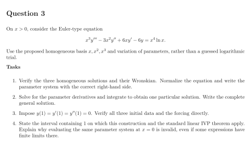
Question 3 – Solution
Strategy. Normalize the Euler operator before solving the derivative equations, and retain its positive-domain restriction.
Step 1: Verify the basis and normalization. For , the left side is . Thus the proposed functions are homogeneous. Their Wronskian is for . Division by gives normalized forcing , so
Step 2: Integrate the solved parameter derivatives. Elimination gives , , . Convenient antiderivatives are Combining gives Integration constants are already represented by the homogeneous terms.
Step 3: Fit and check the initial vector. The particular solution has vector at . The three linear equations for its cancellation give The added terms have vector , verifying the data. For a direct residual check, let . The operator is ; on it gives . With , this is exactly .
Step 4: Respect the regular interval. The normalized coefficients, forcing and nonsingular derivative matrix are valid throughout , the largest such interval containing . At zero the leading coefficient and Wronskian vanish and is undefined. Finite limits of selected terms do not make that parameter system invertible or extend the theorem across zero.